Dataset III - Building an images dataset using SDOML
In this code journey, we'll build a dataset of images using the SDOML dataset, based on the previous general dataset. We'll also create the splits we'll use for training and validation.Once we have a general dataset, we will finetune it to the SDOML dataset. What this entails, in a broad sense is
- Decide exactly how SDOML data will be used
- In particular, we will use hourly SDOML image cutouts of the SHARP regions
- So each sequence shall be defined by two indices which indicate where in a zarr holding the cutouts it starts and ends
- We need to apply certain SDOML related constraints to our dataset
- What we mean is that some images may be missing. Since we're interested in sequences and we don't want to limit our range of possible models, we may have to remove sequences where images are missing
- There are overlaps in the SDOML images that need to be taken into account when splitting the dataset.
Extracting SHARP cutouts from SDOML images
Transforming bounding box coordinates from Heliographic Stonyhurst to pixel coordinated
The first step is to transform the bounding box coordinates from Heliographic Stonyhurst to pixel coordinates. In order to do this, we make use of the FITS header information we downloaded before and of Sunpy to convert coordinates into pixel coordinates. This is done using sunpy's world_to_pixel. It's a process that, at least given how we tackle it, takes quite a long time. Additionally, one should be careful when choosing which corners of the bounding box to use to transform into pixel coordinates. Choosing the wrong ones may result in losing some of the bounding box. The figure below shows how the choice of corner depends on the quadrant of the Sun where the region is
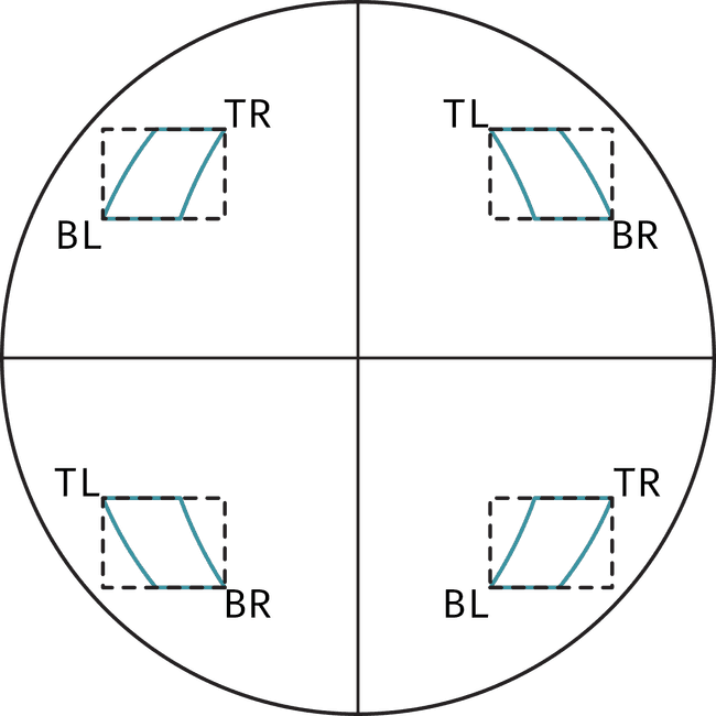
Later on, we'll make use of the largest bounding box width and height as the size for all cutouts. However, it's still important to take care of the quadrant dependence of the corners to ensure we obtain the correct sizes.
While performing the transformation of the more than 2 and a half million bounding boxes in the PROCCESED_HARPS_BBOX table takes a long time (~4 hours on my setup), we have done this before so for this guide we'll just copy over from the previous version of the database (the file where the code to calculate this is at is called 04_convert_bboxes_to_pix). Since in the general dataset we only used bboxes with LONDTMIN > -70 and LONDTMAX < 70 (based on literature values for where the magnetic field measurements can be trusted), we also only consider those for calculation of pixel bounding boxes to reduce the resources needed for this task. We stored the results in a database called pixel_bbox.db. We attach it to our database and copy the values. Note that here we start with a copy of the general dataset database.
conn.execute("DROP TABLE IF EXISTS RAW_HARPS_PIXEL_BBOX;")

# Need to attach the pixel database
conn.execute("ATTACH DATABASE ? AS pixel_values", (PIXEL_DATABASE,))

# Now we need to find the pixel data for each image

conn.execute("""
CREATE TABLE main.RAW_HARPS_PIXEL_BBOX AS
                 SELECT PHPB.harpnum, PHPB.timestamp, PHPB.x_min, PHPB.x_max, PHPB.y_min, PHPB.y_max, PHPB.x_cen, PHPB.y_cen FROM pixel_values.HARPS_PIXEL_BBOX PHPB
                 """)

# Detach the old database

conn.execute("DETACH DATABASE pixel_values")
conn.commit()
Now, as mentioned before, for the pixel bounding boxes we use a fixed width and height. Although the conversion of spherical coordinates to pixel coordinates may yield a different size for the pixel bounding box as it travels the solar disk, we take the largest width and height of the bounding box out of all the timestamps and use it for extracting cutouts. To do this, first we add the maximum width and height to the table HARPS as follows (notice we force the width and heights to be odd so that x_cen,y_cen can be the central pixel of the image as otherwise there's no central pixel)
CREATE TEMP TABLE temp_aggregate AS
SELECT harpnum, MAX(x_max - x_min) as max_width, MAX(y_max - y_min) as max_height
FROM RAW_HARPS_PIXEL_BBOX
GROUP BY harpnum;

UPDATE HARPS
SET pix_width = (
    SELECT max_width + ABS(max_width % 2 - 1)
    FROM temp_aggregate
    WHERE HARPS.harpnum = temp_aggregate.harpnum
),
pix_height = (
    SELECT max_height + ABS(max_width % 2 - 1)
    FROM temp_aggregate
    WHERE HARPS.harpnum = temp_aggregate.harpnum
);

DROP TABLE temp_aggregate;

ALTER TABLE HARPS ADD COLUMN pix_area INTEGER;

UPDATE HARPS
SET pix_area = pix_width * pix_height;
And then we create the final PROCESSED_HARPS_PIXEL_BBOX table as follows
conn.execute("DROP TABLE IF EXISTS PROCESSED_HARPS_PIXEL_BBOX;")

# Then we need to update the values of x_min, x_max, y_min, y_max in PROCESSED_HARPS_PIXEL_BBOX

conn.executescript("""
                    CREATE TABLE IF NOT EXISTS PROCESSED_HARPS_PIXEL_BBOX AS
                    SELECT PHPB.harpnum, PHPB.timestamp,
                    PHPB.x_cen - ((H.pix_width - 1) / 2) AS x_min,
                    PHPB.x_cen + ((H.pix_width - 1) / 2 + 1) AS x_max,
                    PHPB.y_cen - ((H.pix_height - 1) / 2) AS y_min,
                    PHPB.y_cen + ((H.pix_height - 1) / 2 + 1) AS y_max,
                    PHPB.x_cen, PHPB.y_cen
                    FROM RAW_HARPS_PIXEL_BBOX PHPB
                    INNER JOIN HARPS H
                    ON PHPB.harpnum = H.harpnum
                    """)

conn.commit()
And here notice as well we substract 1 from the width and height so it's divisible by 2 and then add the remaining pixel to x_max and y_max, this is again to ensure x_cen and y_cen are at the centre of the image.
Overlaps of pixel bounding boxes
Average values of pixel bounding boxes overlaps are calculated in much the same way as we did for spherical bounding boxes
cur.execute("DROP TABLE IF EXISTS temp_pixel_overlap")

cur.execute("""
CREATE TEMPORARY TABLE temp_pixel_overlap AS
SELECT
    a.harpnum AS harpnum1,
    b.harpnum AS harpnum2,
    a.timestamp AS timestamp,
    100.0 * CASE WHEN a.x_min < b.x_max AND a.x_max > b.x_min AND a.y_min < b.y_max AND a.y_max > b.y_min
        THEN ((MIN(a.x_max, b.x_max) - MAX(a.x_min, b.x_min)) * (MIN(a.y_max, b.y_max) - MAX(a.y_min, b.y_min)))
        ELSE 0
    END / (1.0 * H.pix_area) AS overlap_percent
FROM PROCESSED_HARPS_PIXEL_BBOX a
JOIN PROCESSED_HARPS_PIXEL_BBOX b ON a.timestamp = b.timestamp AND a.harpnum != b.harpnum
JOIN HARPS H ON H.harpnum = a.harpnum;
""")

cur.execute("DROP TABLE IF EXISTS avg_pixel_overlap")
cur.execute("DROP TABLE IF EXISTS PIXEL_OVERLAPS")

cur.executescript("""
CREATE TEMP TABLE avg_pixel_overlap AS
    SELECT tpo.harpnum1 as harpnum_a, tpo.harpnum2 as harpnum_b, AVG(tpo.overlap_percent) AS mean_overlap,
    (100.0 * (CASE WHEN COUNT(tpo.timestamp) > 1
             THEN (COUNT(tpo.timestamp) - 1)
             ELSE (COUNT(tpo.timestamp))
             END
             * 12.0 * 60.0) / (1.0 * NULLIF(strftime('%s', H.end) - strftime('%s', H.start), 0))) AS ocurrence_percentage
    FROM temp_pixel_overlap tpo
    JOIN HARPS H ON H.harpnum = tpo.harpnum1
    WHERE tpo.overlap_percent > 0
    GROUP BY harpnum1, harpnum2;

CREATE TABLE PIXEL_OVERLAPS AS
    SELECT ao.*,
    -- Standard deviation of the overlap
    SQRT(SUM((tpo.overlap_percent - ao.mean_overlap) * (tpo.overlap_percent - ao.mean_overlap)) / CASE WHEN COUNT(tpo.timestamp) > 1 THEN (COUNT(tpo.timestamp) - 1) ELSE 1 END) AS std_overlap
    FROM avg_pixel_overlap ao
    INNER JOIN temp_pixel_overlap tpo ON ao.harpnum_a = tpo.harpnum1 AND ao.harpnum_b = tpo.harpnum2
    GROUP BY harpnum_a, harpnum_b;
""")

conn.commit()
Note here I'm using a case statement to check whether the number of rows with overlap is larger than 1, since I found that for a couple of cases it's equal to one and so the result was null (as we're dividing by 0). I'm aware that this is not done in the spherical coordinates overlap but there weren't any problems there so I may not include it or update later to include it.
Hourly cutouts
While the cadence of our timestamps is 12 minutes, we choose to use images every hour for our dataset. Therefore, it's necessary to create a new table that holds the bounding boxes every hour. This may at first seem like a trivial task. However, given that some images are missing due to quality issues it's not possible to just choose images at a fixed 1 hour interval as in that way we may miss many of them.
CREATE TABLE HOURLY_PIXEL_BBOX AS
SELECT * FROM PROCESSED_HARPS_PIXEL_BBOX PHPBB
WHERE strftime("%M", timestamp) IN ("00", "12", "24")
GROUP BY harpnum, strftime("%Y %m %d %H", timestamp)
In creating the table this way, we give preference to o'clock timestamps but we allow for 12 minutes past or 24 minutes past in that order if the other ones aren't available. While it's true that this means the cadence of the dataset images is not exactly 1 hour, it does make it so the number of images is kept as high as possible.
Loading SDOML image metadata
In order to make it easier the later processing of the dataset, we pre-load metadata of the images in SDOML (by loading HMI images, haven't checked that it's the same for AIA but given the description of SDOML it should be). We want to know what index in each year's zarr each image is at.
What we do is load all the FITS header data for every image, store it in a dictionary with the timestamp as key, and save in pickle format. We can then load the available timestamps into the IMAGES table
# Need to read the SDOML image data
cur.execute("DROP TABLE IF EXISTS IMAGES")
cur.execute("""
CREATE TABLE IMAGES (
  timestamp TEXT NOT NULL UNIQUE,                 -- Unique timestamp for each image
  year INTEGER NOT NULL,                          -- Year the image was captured
  month INTEGER NOT NULL,                         -- Month the image was captured
  day INTEGER NOT NULL,                           -- Day of the month the image was captured
  hour INTEGER NOT NULL,                          -- Hour of the day the image was captured
  minute INTEGER NOT NULL,                        -- Minute of the hour the image was captured
  second INTEGER NOT NULL,                        -- Second of the minute the image was captured
  idx INTEGER NOT NULL                            -- Index to access the image in the zarr format
);
""")


with open(SDOML_TIMESTAMP_INFO, "rb") as f:
    sdoml_timestamp_info = pickle.load(f)

timestamps = list(sdoml_timestamp_info.keys())
indices = [entry["index"] for entry in sdoml_timestamp_info.values()]

i = 0
years = []
months = []
days = []
hours = []
minutes = []
seconds = []
for timestamp in timestamps:
    # Get the year, month, day, hour, minute and seconds from the timestamp
    year = int(timestamp[:4])
    month = int(timestamp[5:7])
    day = int(timestamp[8:10])
    hour = int(timestamp[11:13])
    minute = int(timestamp[14:16])
    second = int(timestamp[17:19])

    years.append(year)
    months.append(month)
    days.append(day)
    hours.append(hour)
    minutes.append(minute)
    seconds.append(second)

new_data = [(timestamp, year, month, day, hour, minute, second, idx) for timestamp, year, month, day, hour, minute, second, idx in zip(timestamps, years, months, days, hours, minutes, seconds, indices)]

cur.executemany("INSERT INTO IMAGES (timestamp, year, month, day, hour, minute, second, idx) VALUES (?, ?, ?, ?, ?, ?, ?, ?) ON CONFLICT(timestamp) DO NOTHING", new_data)
conn.commit()

del sdoml_timestamp_info, timestamps, indices, years, months, days, hours, minutes, seconds, new_data
gc.collect()
Considering the distribution of areas
So, when it comes to the overlaps there are some things we need to worry about.
-
We don't want positive class examples to be overlaping with negative class examples or viceversa, as this would mean we show two examples with common features to the model but with different labels. So, it may be worth to just look at which regions with negative labels overlap with positive regions (those that have at least one CME associated with them) and just remove them.
-
We should see if there's any bias in the size of the regions that produce CMEs and those that don't, and try to correct it.
So let's begin by looking at how many non positive regions overlap with a positive region. We query the overlaps of cases where a non-CME region overlaps with a CME region.
df = pd.read_sql("""
WITH cme_info AS (
SELECT
            PO.harpnum_a,
            PO.harpnum_b,
            CASE WHEN MAX(FCHA.harpnum) IS NULL THEN 0 ELSE 1 END AS harpnum_a_cme,
            CASE WHEN MAX(FCHA2.harpnum) IS NULL THEN 0 ELSE 1 END AS harpnum_b_cme,
			mean_overlap,
			ocurrence_percentage

FROM PIXEL_OVERLAPS PO
LEFT JOIN FINAL_CME_HARP_ASSOCIATIONS FCHA ON
PO.harpnum_a = FCHA.harpnum
LEFT JOIN FINAL_CME_HARP_ASSOCIATIONS FCHA2 ON
PO.harpnum_b = FCHA2.harpnum
GROUP BY PO.harpnum_a, PO.harpnum_b)

SELECT * FROM cme_info
WHERE harpnum_a_cme != harpnum_b_cme
ORDER BY mean_overlap ASC
""", conn)
And if we plot the distribution of overlap percents vs ocurrence percentage we get
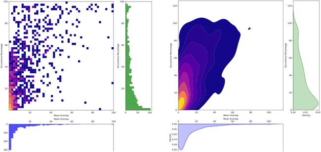
So luckily, it seems like most overlaps are small and don't last long. However, there are some cases when that is not the case. To keep things simple, we can just say that any non-CME region that overlaps with a CME regions more than 30% (either way, so either the non-CME overlaps 30% of its area or the CME one does) for more than 30% of their lifetime, we will drop the non-CME region.
I agree that this is no elegant solution, but for now I'd prefer to keep things simple. The good thing is that if anything, this issue will make the model perform worse so it won't make us believe it has a performance better than the real one. That would be a problem if we don't tackle the overlaps in the splits correctly. However, for this overlap between yes/no CME regions, it can only confuse the model and make it perform worse, not better.
So we do as follows
# Add columns harpnum_a_cme and harpnum_b_cme to PIXEL_OVERLAPS

try:
    cur.executescript("""
    ALTER TABLE PIXEL_OVERLAPS ADD COLUMN harpnum_a_cme INTEGER;
    ALTER TABLE PIXEL_OVERLAPS ADD COLUMN harpnum_b_cme INTEGER;
    """)
# Maybe they already exist
except sqlite3.OperationalError:
    pass

cur.execute("""
WITH cme_info AS (
SELECT
            PO.harpnum_a,
            PO.harpnum_b,
            CASE WHEN MAX(FCHA.harpnum) IS NULL THEN 0 ELSE 1 END AS harpnum_a_cme,
            CASE WHEN MAX(FCHA2.harpnum) IS NULL THEN 0 ELSE 1 END AS harpnum_b_cme,
			mean_overlap,
			ocurrence_percentage

FROM PIXEL_OVERLAPS PO
LEFT JOIN FINAL_CME_HARP_ASSOCIATIONS FCHA ON
PO.harpnum_a = FCHA.harpnum
LEFT JOIN FINAL_CME_HARP_ASSOCIATIONS FCHA2 ON
PO.harpnum_b = FCHA2.harpnum
GROUP BY PO.harpnum_a, PO.harpnum_b)

UPDATE PIXEL_OVERLAPS
SET harpnum_a_cme = (
SELECT harpnum_a_cme FROM cme_info
WHERE PIXEL_OVERLAPS.harpnum_a = cme_info.harpnum_a AND PIXEL_OVERLAPS.harpnum_b = cme_info.harpnum_b
),
harpnum_b_cme = (
SELECT harpnum_b_cme FROM cme_info
WHERE PIXEL_OVERLAPS.harpnum_a = cme_info.harpnum_a AND PIXEL_OVERLAPS.harpnum_b = cme_info.harpnum_b
)
            """)

conn.commit()
So now we can get a list of the HARPNUMs that will sadly be ignored in the final dataset by doing
cur.execute("""
CREATE TEMP TABLE ignore_harps AS
    SELECT
       CASE
           WHEN harpnum_a_cme THEN harpnum_b
           ELSE harpnum_a
       END AS to_ignore
FROM PIXEL_OVERLAPS
WHERE harpnum_a_cme != harpnum_b_cme
  AND mean_overlap > 30
  AND ocurrence_percentage > 30
ORDER BY harpnum_a, harpnum_b ASC;
""")
So, with that out of the way. We can now take a look at the distribution of areas of the regions that produce CMEs and those that don't. I will consider all regions now as I don't care about overlaps for this. We do this as follows
df = pd.read_sql("""
WITH SELECTED_HARPS AS (
                 SELECT DISTINCT harpnum FROM HOURLY_PIXEL_BBOX
)
SELECT
                 *,
                 CASE WHEN FCHA.cme_id IS NULL THEN 0 ELSE 1 END AS has_cme
FROM HARPS
LEFT JOIN FINAL_CME_HARP_ASSOCIATIONS FCHA ON HARPS.harpnum = FCHA.harpnum
INNER JOIN SELECTED_HARPS SH ON HARPS.harpnum = SH.harpnum
GROUP BY HARPS.harpnum
""", conn)

df["norm_pix_area"] = 100 * df["pix_area"] / (100 * 100)
Which, plotting both distributions we get
So well... quite different distributions. Now, because of this it may be that the model (even though we resize images to same size), learns to distinguish CME regions based only on telltale signs about the original size of the image. Not something we'd really like to happen. Now, one thing we can do is try to ajust the distrubition of non-cme regions by undersampling from it like this
# Create bins for the 'No CME' data based on 'norm_pix_area'
labels = range(len(hist_bins) - 1)
df['bin'] = pd.cut(df['norm_pix_area'], bins=hist_bins, labels=labels)

# Separate 'Yes CME' and 'No CME' data
df_yes = df[df['has_cme'] == 1]
df_no = df[df['has_cme'] == 0]

df_yes_cme_counts = df_yes['bin'].value_counts()
df_no_cme_counts = df_no['bin'].value_counts()
# Assume df_yes_cme_counts and df_no_cme_counts are the counts of 'Yes CME' and 'No CME' in each bin
# You can get this information using something like df[df['has_cme'] == 1]['bin'].value_counts()

# Calculate the desired number of 'No CME' in each bin based on the 'Yes CME' distribution
desired_no_cme_counts =  5 * df_yes_cme_counts  # Or some other criteria

# Calculate frac for each bin
frac_per_bin = desired_no_cme_counts / df_no_cme_counts

# Clip the frac values to be between 0 and 1
frac_per_bin = frac_per_bin.clip(0, 1)
frac_per_bin.replace(np.nan, 1, inplace=True)

# Perform stratified sampling
sampled_df_no = df_no.groupby('bin').apply(lambda x: x.sample(frac=frac_per_bin.get(x.name, 1)))

# Remove index level added by groupby and sampling
sampled_df_no.reset_index(drop=True, inplace=True)

# Concatenate the sampled 'No CME' data with the 'Yes CME' data to get the balanced dataset
df_balanced = pd.concat([df_yes, sampled_df_no])

# Remove the 'bin' column as it's no longer needed
df_balanced.drop(columns=['bin'], inplace=True)

df_balanced.reset_index(drop=True, inplace=True)
Where our objective in the snippet above is to have five times more non-CME regions than CME regions but make them follow the same distribution over area. However, this is impossible as there are just not enough non-CME regions for all the bins where there are CME regions to cover for all the needed numbers. Meanwhile, there are way more regions in the low area numbers. As a result we get the following distribution
So it's a bit better, more similar between eachoter. The bad part? While we started with 3079 non-CME regions, now we have only 984. So, in order to make the distributions more similar we lose a lot of the non-CME regions.
What's best? Should we just use the biased distribution? What about the super small regions? Do we just get rid of them? If we decide to go through with the biased distribution we can always check after training if the model is biased to making decision based solely on the original size of the image. For example, we could take one of the big CME regions, artificially reduce its size before giving it to the model and see if it changes the prediction. I think that would be a good indication it's biased. But, what about the super small regions?
Let's look at the distribution only over 0-20% (this is % of the number of pixels a 100x100 image has)
Big number of regions don't even have 5% of that, which is the equivalent of being smaller than an image of 22x22. Lets see what it would look like to have 16x16 image rescaled to 256x256
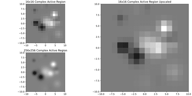
On the bottom left you can compare to what it would look like to have it in original 256x256 resolution. So, doesn't look pretty but also it looks better than I expected. Perhaps it's ok to keep these small ones? Let's see with a much more complex one
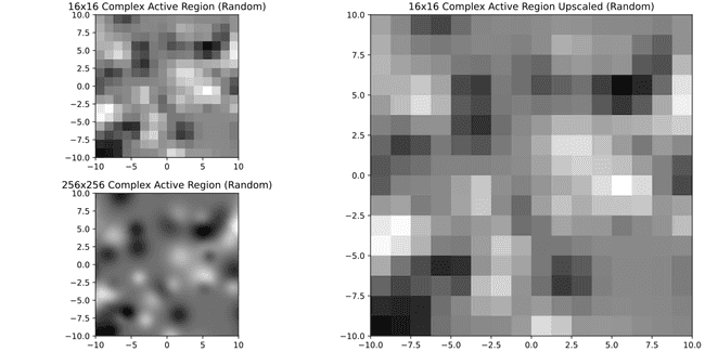
Well... not so nice anymore. Meanwhile if we were to require 32x32 or 64x64

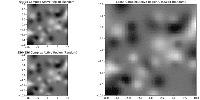
It's much better. Just for curiosity here's 8x8
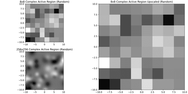
Well. Problem is all of this is subjective, in principle it would be more important to know what's the size of features that can be important for forecasting CMEs, see what their size would be in pixels in a SDOML image and then decide based on that. Since I don't have that, I may have to just decide that images that have less pixels than say a 16x16 image are not useful. In doing so, we lose 1333 no CME regions and 7 CME regions. If I do that, the new distribution is
df["eq_side"] = np.sqrt(df["pix_area"])

df["big_enough"] = df["eq_side"] > 16

big_enough_regions = df[df["big_enough"]]
So as a side effect we've also made the distributions a bit more similar.
So, removing the overlaps and the small regions we have
| Overlap Rejected | Size Rejected | Accepted | Total | |
|---|---|---|---|---|
| CME | 0 | 7 | 462 | 469 |
| No CME | 132 | 1272 | 1675 | 3079 |
| Total | 132 | 1279 | 2137 | 3548 |
So we create a list of accepted harps with
cur.execute("DROP TABLE IF EXISTS ACCEPTED_HARPS")
cur.execute("""
CREATE TABLE ACCEPTED_HARPS AS
            SELECT DISTINCT H.harpnum FROM HARPS H
            INNER JOIN HOURLY_PIXEL_BBOX HPB ON H.harpnum = HPB.harpnum
            LEFT JOIN ignore_harps ih ON H.harpnum = ih.to_ignore
            WHERE H.pix_area > 256 AND ih.to_ignore IS NULL
""")

conn.commit()
Creating the dataset
Image indices
We begin by finding the zarr index for each of the entries in the HOURLY_PIXEL_BBOX table. This is done as follows
cur.execute("ALTER TABLE HOURLY_PIXEL_BBOX ADD COLUMN zarr_index INTEGER;")

# Select all harpnums
cur.execute("""
SELECT DISTINCT harpnum FROM HOURLY_PIXEL_BBOX
""")

harpnums = cur.fetchall()

# Create index for harpnum, index for
# faster access

cur.execute("""
CREATE INDEX IF NOT EXISTS idx_hourly_pixel_bbox_harpnum_timestamp ON PROCESSED_HARPS_PIXEL_BBOX (harpnum, timestamp)
""")

# Now we go through each harpnum and find the zarr index for each timestamp
for harpnum in harpnums:
    harpnum = harpnum[0]

    # Open the zarr DirectoryStore
    zarr_path = os.path.join(ZARR_BASE_PATH, f"{harpnum}")

    zarr_store = zarr.DirectoryStore(zarr_path)

    # Open the zarr group
    root = zarr.group(store=zarr_store, overwrite=False)

    # Get the timestamps from the zarr group
    attrs = root.attrs.asdict()

    timestamps = attrs["timestamps"]

    # Now we need to update each entry in the table with the zarr index

    for i, timestamp in enumerate(timestamps):
        cur.execute("""
        UPDATE HOURLY_PIXEL_BBOX
        SET zarr_index = ?
        WHERE harpnum = ? AND timestamp = ?
        """, (i, harpnum, timestamp))

conn.commit()
Updating the sequences
Now we must go through each of the sequences of the general dataset.
For now, we'll do as follows
-
Take all sequences with 24 images, as they're not missing any
-
Take also sequences with 23 images (and we will just repeat the last image before the gap to fill it) but only if the missing image is not the last one.
Why? Because the last image is essential for defining the label (CME X hours after last image), so losing it would break the labels.
In practice we can do this by choosing the slices with 23 images and last image being 30 mins before then end of the slice.
There are smarter (or maybe less smart, who knows) ways to go about this. For example
- We could train a model to fill missing images by providing it with the image before it and after it.
- Time consuming
- Would it work?
- What about gaps larger than one
- We could just repeat the last image
- Would it work?
- How would it affect the output?
So while there are other ways, I have no guarantee they will work better. For now I'm going with the easiest. Will I lose many slices? Yes. But, for now we have to keep things simple and only complicate them if needed.
So we do as follows.
cur.executescript("""
DROP TABLE IF EXISTS slice_img_counts;
DROP TABLE IF EXISTS SDOML_DATASET;
""")

cur.executescript("""
CREATE TEMP TABLE slice_img_counts AS
SELECT slice_id, COUNT(*) AS img_count, MIN( zarr_index ) AS start_index, MAX( zarr_index ) AS end_index, MIN(timestamp) AS start_image, MAX(timestamp) AS end_image
FROM GENERAL_DATASET
INNER JOIN HOURLY_PIXEL_BBOX HPB ON GENERAL_DATASET.harpnum = HPB.harpnum AND GENERAL_DATASET.obs_start <= HPB.timestamp AND GENERAL_DATASET.obs_end >= HPB.timestamp
GROUP BY slice_id;

CREATE TABLE SDOML_DATASET AS
SELECT GD.*, SIC.img_count, SIC.start_index, SIC.end_index, SIC.start_image, SIC.end_image, SIC.img_count as img_count
FROM GENERAL_DATASET GD
INNER JOIN slice_img_counts SIC ON GD.slice_id = SIC.slice_id
INNER JOIN ACCEPTED_HARPS AH ON GD.harpnum = AH.harpnum
WHERE
SIC.img_count = 24 OR
(SIC.img_count = 23 AND ((strftime(GD.obs_end) - strftime(SIC.end_image)) / 60.0) <= 30)
""")

conn.commit()
So, in the end we have 254218 individual sequences. Out of those, 21754 are positive while 232464 are negative. So, due to SDOML constraints (overlaps, size in pixels and missing images) images we've lost 6083 positive rows and 113122 negative rows.
Note however that these rows are not independent, if we consider only individual HARPNUM-CMEID pairs, we have 350 pairs coming from 281 HARPs regions. Meanwhile, there are 1633 non-CME regions
Creating the splits in the database
The final step it to separate the dataset into 4 splits. Our objective is to create the splits such that
- All HARPs that overlap fall within the same split, so as to prevent data leakage between training and validation/test sets.
- Ensure that there's a roughly equal number of CMEs (and regions) in each split for each verification score.
Before starting, and to make our task easier, we create two tables calles SDOML_HARPS and SDOML_CME_HARPS_ASSOCIATIONS which hold only the HARPs and CMEs that appear in the SDOML_DATASET table. That is, only the ones that have made it to the final dataset.
cur.execute("DROP TABLE IF EXISTS SDOML_HARPS")
cur.execute("DROP TABLE IF EXISTS available_harps")
cur.execute("DROP TABLE IF EXISTS SDOML_CME_HARPS_ASSOCIATIONS")
cur.execute("DROP TABLE IF EXISTS available_cmes")

cur.executescript("""
CREATE TEMP TABLE available_harps AS
SELECT DISTINCT harpnum FROM SDOML_DATASET;

CREATE TABLE SDOML_HARPS AS
SELECT H.* FROM HARPS H
INNER JOIN available_harps AH ON H.harpnum = AH.harpnum;

CREATE TEMP table available_cmes AS
SELECT DISTINCT cme_id FROM SDOML_DATASET;

CREATE TABLE SDOML_CME_HARPS_ASSOCIATIONS AS
SELECT FCHA.* FROM FINAL_CME_HARP_ASSOCIATIONS FCHA
INNER JOIN SDOML_HARPS SH
ON FCHA.harpnum = SH.harpnum
INNER JOIN available_cmes AC
ON FCHA.cme_id = AC.cme_id;
""")
Overlap groups
To ensure we satisfy the first condition, we create a SDOML_GROUPS table that holds the id for groups which contain HARPs that overlap (or in the case of a HARP that doesn't overlap, it contains only that HARP). Every HARPNUM has an associated group_id. The way we go about this is using the networkx package in Python. Essentially, each HARPNUM is a node in a graph and we connect nodes that overlap. Then, this package can give us directly the groups of overlapping HARPs. In the figure below is a simple example of what this would look like visually
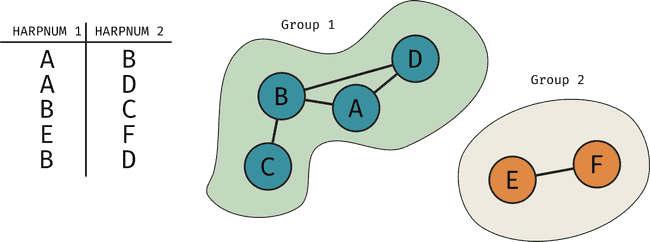
In code, we do this
harps_df = pd.read_sql("""SELECT harpnum FROM SDOML_HARPS""", conn)
overlaps_df = pd.read_sql("""
SELECT PO.harpnum_a, PO.harpnum_b
FROM PIXEL_OVERLAPS PO
INNER JOIN SDOML_HARPS SH1 ON
PO.harpnum_a = SH1.harpnum
INNER JOIN SDOML_HARPS SH2 ON
PO.harpnum_b = SH2.harpnum
WHERE mean_overlap > 5 AND ocurrence_percentage > 5""", conn)

# Create an empty graph
G = nx.Graph()

# Add edges to the graph based on the overlaps table
for idx, row in overlaps_df.iterrows():
    G.add_edge(row['harpnum_a'], row['harpnum_b'])

# Find connected components
connected_components = list(nx.connected_components(G))

# Create a dictionary to store the group for each harpnum
group_dict = {}
group_size = []

used_harps = set()
for group_num, component in enumerate(connected_components):
    group_size.append((group_num, len(component)))

    for harpnum in component:
        if harpnum in used_harps:
            raise ValueError(f"The harpnum {harpnum} is in more than one group")
        used_harps.add(harpnum)
        group_dict[harpnum] = group_num

# Now, for all the harps that didn't get a group we keep assigning groups

group_num = len(group_dict)

for harpnum in harps_df['harpnum']:
    if harpnum not in group_dict:
        if harpnum in used_harps:
            raise ValueError(f"The harpnum {harpnum} is in more than one group")
        used_harps.add(harpnum)

        group_num += 1
        group_dict[harpnum] = group_num
        group_size.append((group_dict[harpnum], 1))

harps_group = [(group_dict[harpnum], int(harpnum)) for harpnum in group_dict.keys()]

try:
    cur.execute("ALTER TABLE SDOML_HARPS ADD COLUMN group_id INTEGER;")
except sqlite3.OperationalError as e:
    if "duplicate column name: group_id" == str(e):
        pass
    else:
        raise e

cur.executemany("""
UPDATE SDOML_HARPS
SET group_id = ?
WHERE harpnum = ?
""", harps_group)

cur.execute("DROP TABLE IF EXISTS SDOML_GROUPS")

cur.execute("""
CREATE TABLE SDOML_GROUPS (
    group_id INTEGER PRIMARY KEY,
    group_size INTEGER,
    n_level_1 INTEGER,
    n_level_2 INTEGER,
    n_level_3 INTEGER,
    n_level_4 INTEGER,
    n_level_5 INTEGER
)
""")

cur.executemany("""
INSERT INTO SDOML_GROUPS (group_id, group_size) VALUES (?, ?)
                """, group_size)

conn.commit()
Obviously, for the dataset we're interested in knowing how many CMEs of each level there are in each group. So we do as follows
groups = pd.read_sql("""
SELECT SH.harpnum, SH.group_id, SCHA.verification_score FROM SDOML_HARPS SH
INNER JOIN SDOML_CME_HARPS_ASSOCIATIONS SCHA
ON SCHA.harpnum = SH.harpnum
""", conn)

# Count the occurrences of each verification_score within each group
count_df = groups.groupby(['group_id', 'verification_score']).size().reset_index(name='count')


# Pivot the table to have verification_scores as columns
pivot_df = count_df.pivot(index='group_id', columns='verification_score', values='count').fillna(0).reset_index()

all_group_ids_df = pd.read_sql("SELECT DISTINCT group_id FROM SDOML_GROUPS", conn)

# Merge with pivot_df, filling in missing values with zeros
final_df = pd.merge(all_group_ids_df, pivot_df, on='group_id', how='left').fillna(0)

# Generate the tuples
result_tuples = [tuple(row) for row in final_df.itertuples(index=False, name=None)]

# Need group_id to be the last element of the tuple

result_tuples = [(int(t[1]), int(t[2]), int(t[3]), int(t[4]), int(t[5]), int(t[0])) for t in result_tuples]


cur.executemany("""
UPDATE SDOML_GROUPS
SET n_level_1 = ?,
    n_level_2 = ?,
    n_level_3 = ?,
    n_level_4 = ?,
    n_level_5 = ?
WHERE group_id = ?
""", result_tuples)

conn.commit()
And finally we make the splits. Now, it seems this is no easy task and we can only get to an approximate solution using a heuristic method, in particular greedy algorithm. What this means is we decide on the importance of different numbers. So, the most important is having level 1 verified CMEs split correctly, then level 2 and so on and then at the end having the number of regions split well enough. Then, we go through the list of all attributes. For each attribute, we go through the list of all groups (that have not yet been assigned) and sort it by the largest number of that attribute. Then, one by one we assign each group to the split that has the least number of that attribute (sorting again after adding each group). We do this until all groups have been assigned. In code, we do this as follows
UPDATE: Number of splits doubled
Below, I make 10 splits. The idea is to have 5 splits and each split have 2 subsplits. Why? Because I'm not sure yet how I will split the data into training, test and validation. I could do 60/20/20 but that may not leave enough data for training. If that's the case then I could do 80/10/10 by considering a single split for test/validation and using one subsplit for each.
# Now time to make the actual splits
df = pd.read_sql("""
SELECT group_id, n_level_1, n_level_2, n_level_3, n_level_4, n_level_5, group_size FROM SDOML_GROUPS
""", conn)

df.set_index('group_id', inplace=True)

# Initialize splits
N_SPLITS = 10
splits = {i: {'group_ids': [], 'totals': {col: 0 for col in df.columns if col != 'group_id'}} for i in range(1, N_SPLITS + 1)}

# Sort by each n_level_x column in descending order. We sort first level1, level2 ... until at the end group_size
df.sort_values(by=[col for col in df.columns if col != 'group_id'], ascending=False, inplace=True)

attributes = ["n_level_1", "n_level_2", "n_level_3", "n_level_4", "n_level_5", "group_size"]

# We go through the attributes in this order (order of priority)

used_groups = set()

for attribute in attributes:
    # Sort the df by the attribute

    assign_df = df[df[attribute] > 0].sort_values(by=[attribute], ascending=False)

    # Now we go row by row

    for group_id, row in assign_df.iterrows():
        if group_id in used_groups:
            raise ValueError(f"Group {group_id} already used")
        # Sort the splits to get the one with the lowest total for the attribute

        sorted_splits = sorted(splits.keys(), key=lambda x: splits[x]['totals'][attribute])

        # Get the split with the lowest total for the attribute

        split = sorted_splits[0]

        # Add the group_id to the split

        splits[split]['group_ids'].append(group_id)

        # Update the totals for the split

        for col in df.columns:
            if col != 'group_id':
                splits[split]['totals'][col] += row[col]

        # Take the group_id out of the df and assign_df

        df.drop(group_id, inplace=True)
        used_groups.add(group_id)

# Now, we did 10 splits because we want 5 splits, each divided into two
# So there will be a split and then a subsplit
# So we need to map every two subsplits to the same split

try:
    cur.execute("ALTER TABLE SDOML_GROUPS ADD COLUMN split INTEGER;")
except sqlite3.OperationalError as e:
    if "duplicate column name: split" == str(e):
        pass
    else:
        raise e

try:
    cur.execute("ALTER TABLE SDOML_GROUPS ADD COLUMN subsplit INTEGER;")
except sqlite3.OperationalError as e:
    if "duplicate column name: subsplit" == str(e):
        pass
    else:
        raise e

for split, split_dict in splits.items():
    group_ids = split_dict['group_ids']
    subsplit_number = split % 2 + 1
    split_number = (split + 1) // 2
    cur.executemany("UPDATE SDOML_GROUPS SET split = ?, subsplit = ? WHERE group_id = ?", [(split_number, subsplit_number, group_id) for group_id in group_ids])

conn.commit()


# Now time to make the actual splits
df = pd.read_sql("""
SELECT group_id, n_level_1, n_level_2, n_level_3, n_level_4, n_level_5, group_size FROM SDOML_GROUPS
""", conn)

df.set_index('group_id', inplace=True)
And at the end we can print some info about the resulting splits
# Print slices info
df = pd.read_sql("""
SELECT * FROM SDOML_DATASET
INNER JOIN SDOML_HARPS ON SDOML_DATASET.harpnum = SDOML_HARPS.harpnum
INNER JOIN SDOML_GROUPS ON SDOML_HARPS.group_id = SDOML_GROUPS.group_id
""", conn)

nrows = df.groupby(['split', 'subsplit', 'label']).size().reset_index(name='counts')

n_rows_pivot = pd.pivot_table(nrows, values='counts', index=['split','subsplit'], columns=['label'], aggfunc=np.sum)

# Print in markdown
print("N Positive and negative rows")
print(n_rows_pivot.to_markdown())

# Rename the columns to neg_row and pos_row

n_rows_pivot.rename(columns={0: "neg_row", 1: "pos_row"}, inplace=True)

# Now the number of CMEs per split by verification level

ncmes = df[df["label"].astype(bool)].drop_duplicates(subset=['cme_id']).groupby(['split', 'subsplit', 'verification_level']).size().reset_index(name='counts')

ncmes_pivot = pd.pivot_table(ncmes, values='counts', index=['split', 'subsplit'], columns=['verification_level'], aggfunc=np.sum)

# To markdown
print("N cmes by verif level per split")
print(ncmes_pivot.to_markdown())

# Rename columns to n_cme_level_x

ncmes_pivot.rename(columns={1: "n_cme_level_1", 2: "n_cme_level_2", 3: "n_cme_level_3", 4: "n_cme_level_4", 5: "n_cme_level_5"}, inplace=True)

# Now number of cme productive and non cme productive regions per split

nreg = df.sort_values(by="label", ascending=False).drop_duplicates(subset=['harpnum'], keep="first").groupby(['split', 'subsplit', 'label']).size().reset_index(name='counts')

nreg_pivot = pd.pivot_table(nreg, values='counts', index=['split', 'subsplit'], columns=['label'], aggfunc=np.sum)

# To markdown

print("N regions per subsplit with and without CME")
print(nreg_pivot.to_markdown())

# Rename columns to pos_reg and neg_reg

nreg_pivot.rename(columns={0: "neg_reg", 1: "pos_reg"}, inplace=True)

# Now combine all pivots, which should share the same index
combined_pivot = pd.concat([n_rows_pivot, ncmes_pivot, nreg_pivot], axis=1)


conn.close()
Which results
| neg_row | pos_row | n_cme_level_1 | n_cme_level_2 | n_cme_level_3 | n_cme_level_4 | n_cme_level_5 | neg_reg | pos_reg | |
|---|---|---|---|---|---|---|---|---|---|
| (1, 1) | 22683 | 3191 | 4 | 3 | 5 | 18 | 14 | 159 | 33 |
| (1, 2) | 22380 | 2632 | 4 | 3 | 5 | 19 | 14 | 157 | 35 |
| (2, 1) | 21085 | 3062 | 3 | 3 | 5 | 18 | 14 | 156 | 36 |
| (2, 2) | 23257 | 2871 | 4 | 3 | 5 | 18 | 14 | 159 | 33 |
| (3, 1) | 22817 | 2869 | 3 | 3 | 5 | 18 | 14 | 158 | 33 |
| (3, 2) | 22049 | 3600 | 3 | 3 | 5 | 18 | 14 | 158 | 33 |
| (4, 1) | 22277 | 2816 | 3 | 3 | 4 | 18 | 14 | 156 | 35 |
| (4, 2) | 22111 | 3058 | 3 | 3 | 5 | 18 | 14 | 155 | 36 |
| (5, 1) | 23056 | 2980 | 3 | 2 | 4 | 18 | 13 | 159 | 32 |
| (5, 2) | 22305 | 3077 | 3 | 3 | 4 | 18 | 14 | 159 | 32 |
So quite nicely distributed.
Data reduction summary
| Step | Substep | CMEs | SHARP regions |
|---|---|---|---|
| Starting point | 498 | 3551 | |
| Pre-processing | Need images and hourly | 498 | 3548 |
| Pre-processing | Removing overlaps | 498 | 3416 |
| Pre-processing | Remove small harps | 493 | 2137 |
| Adjust General Dataset | 429 | 1914 |
